Welcome to the IMPACT documentation. Here you will learn all there is to know about IMPACT and get a quick start guide on how to use the different tools.
The software tool can be used for multiple types of analysis. Next to investigation of the active metabolism in any kind of sample that was analysed with LC MS, comparisons of the active metabolism between different samples can be made. Such samples can be representing different tissues from the same species, or different developmental stages of the same or different tissues from the same species as well as samples from genetically different species or varieties, like different production strains. Alternatively, also samples representing different treatments can be analysed. Treatments to be used could be changes in growth conditions, e.g. by application of biotic or abiotic stress, as well as application of chemicals, like growth promoters, drugs, herbicides, pesticides or fungicides.
The analysis workflow can be optimized in the future in multiple ways. Potential ways to improve the annotation part of the workflow are including more or newer versions of MS2 spectral libraries, or implementing other algorithms or datasets that can be used to annotate features from an untarget LC measurement. Another way to improve the workflow is by enabling the inclusion of isotopolome data generated by different technologies in the workflow, like gaschromatography coupled to mass spectroscopy.
The IMPACT demo dataset provides an example of how to use the Integrative Metabolomics Platform for Analysis, Contextualization, and Targeting (IMPACT) for stable-isotope labeling experiments. The data includes the following two bacterial strains:
Each strain was measured under four conditions:
Contents of the Demo Data:
MID files (*_fast.csv): A smaller version is available.
Pathway JSON file: Optional, enables pathway mapping.
Precomputed network graphs (*_small.json): Already computed graphs can be uploaded using the switch.
If you wish to include metabolite annotation: Upload lib.csv from preprocessing/step2/.
To enable MS2 annotation: Upload raw MS2 files.
Adjust Parameters (Optional)
Submit for Processing
The "Targeted Analysis" tool can calculate Mass Isotopomer Distributions (MIDs) for the given peak intensities or areas of every measured metabolite. To calculate MIDs you need to upload a CSV or TSV file with the following columns:
| reference | name | intensity | mass_isotopomer | replicate | experiment | condition |
|---|---|---|---|---|---|---|
| A unique sample identifier. | The name of the respective metabolite. | Intensity of the metabolite. | The mass isotopomer in M+0 or m+0 form. | Replicate number of the sample. | Experiment identifier. Experiments are separated into different figures. | Condition identifier. Conditions are shown in the same figure. |
| Sample_1 | Pyruvate | 1000000 | M+0 | 1 | 1000 | T0 |
After you successfully uploaded your data you will be redirected to the MID data page.
The MID data page displays by default the calculated Mass Isotopomer Distributions for the first metabolite and first experiment. With the metabolite and experiment selectors you can switch between the different metabolites and experiments. You can zoom into the data by dragging a rectangle above the data you want to enlarge. To zoom out of the data just double click into the graph. Clicking on a condition in the legend disables or enables them respectively. Finally you can download the calculated MIDs with the "Download CSV" button.
LC-MS Preprocessing can be done with the file formats mzXML, mzML, or mzData. Just upload your files or drag and drop the files into the upload window. Additionally you can upload a group.json file. This is an optional file used for grouping during preprocessing. Each unique condition should get a unique group, which is mapped to the conditions raw files. Below you can see an example:
{
  "20min_replicate1.mzMl": "20min",
  "20min_replicate2.mzMl": "20min",
  "1hour_replicate1.mzMl": "1hour",
  "1hour_replicate2.mzMl": "1hour"
}
After uploading the raw files you can delete each file separately, delete all of them to start new or upload the files to the server and continue with parameter selection.
Parameters can be chosen for a multitude of functions, specifically "peak picking", "peak alignment", "peak grouping", "MS1 Annotation", and optionally "Library Annotation" and "MS2 Annotation".
Peak pickings most important parameters are both the min and max peak width, as well as the ppm. The ppm is dependent on the instrument used and in practice often higher than given by the instrument manufacturer. The peak widths can approximately be determined by looking at the spectra and choosing half the average width in seconds and double the average width for min and max respectively. Integrate chooses the integration method, where 2 is more accurate but prone to noise error. Snthresh, noise, and prefilter options are all related to noise filtering. Sntresh is the signal to noise ratio, noise the minimum intensity required for peak picking and prefilter filters peaks for the first step if they do not have at least the given counts peak intensities.
Peak alignment only has two options, minFraction defines the minimum number of required fractions of samples in which peaks for the peak group were identified. For example in the above "20 min" group if minFraction is set to 1 both samples need to have the peak present, for 0.5 minFraction only one sample needs to have the peak. Span determines the degree of smoothing for the loess function and can be left as is.
Peak grouping or correspondence groups multiple peaks from the same type of compounds across samples to form features. Here there are 3 options, bw or bandwidth changes the smoothness of the density function and should be evaluated based on the peak widths of the peak picking step. A bw of slightly lower than the min peak width should be ideal but might have to be changed in different runs to get optimal results. MinFraction has the same function as in the alignment step. BinSize defines the maximal acceptable difference in m/z values for peaks to be considered grouped. The value depends on the resolution and noise of the LC-MS instrument.
MS1 Annotation is the first step in the annotation process. It annotates features based on accurate m/z masses. Polarity is a selector for the used LC-MS polarity (either negative or positive), while Adducts is a choice of multiple possible adducts for each polarity that can be chosen. Ppm again is the accuracy with which to annotate these compounds.
Library annotation is a instrument specific annotation based on measured standards, accurate masses and retention times. To perform library annotation a csv file in the below format needs to uploaded. Ppm and toleranceRt can be chosen based on the expected m/z and retention time differences.
| name | id | formula | exactmass | rt |
|---|---|---|---|---|
| The name of the respective metabolite. | A unique metabolite identifier. | Formula of the respective metabolite. | Exact mass of the metabolite. | Expected retention time in seconds. |
| Pyruvate | 65 | C3H4O3 | 87.008220 | 120 |
MS2 Annotation can be performed if unlabeled MS2 data was measured. Here MS2 peaks are mapped to the LC-MS features and then compared to a MS2 spectra database. To use MS2 annotation raw files need to be uploaded. Ppm and tolerance are both 2 options to adjust potential m/z differences. ToleranceRt again is the difference between MS2 and LC-MS features retention time. ScoreThreshold is the threshold for MS2 database matches. Lastly, requirePrecursor should be used to require a precursor match before spectra matching. If it is disabled the hits will increase but the wait time will also greatly increase.
Finally, after all the parameters are changed the job can be submitted which redirects the user to a different job queue page.
Mass Isotopomer Distribution (MID) calculation requires 3 files, a "Feature Intensity" and a "Feature Annotation" file (which can be used from the previous step), as well as a "Group" file. The files should have the following format.
Feature Intensity (from Preprocessing): The Feature Intensity file should hold all feature intensities detected during preprocessing. Each column represents 1 sample where the column name is the file name. Each row represents a single feature which can be mapped onto the annotation file (so row 1 in the intensity and annotation file are the same feature).
| 20min_replicate1.mzMl | 20min_replicate2.mzMl | ... |
|---|---|---|
| Intensity of feature 1 for sample 1. | Intensity of feature 1 for sample 2. | ... |
| Intensity of feature 2 for sample 1. | Intensity of feature 2 for sample 2. | ... |
Feature Annotation (from Preprocessing): The Feature Annotation file should also map to the same feature in each row as the Feature Intensity file.
| rtmed | mzmed | name | id | formula |
|---|---|---|---|---|
| Retention time of each feature. | Accurate mass of each feature. | Annotation or feature name. | Unique feature identifier. | Predicted feature formula. |
| 120 | 87.008220 | FT00001 | 65 | C3H4O3 |
Group File: The group file is a reference information file for each sample. Each row represents a single sample.
| file_name | labeling | experiment | condition |
|---|---|---|---|
Sample file name which is identical to one sample in the feature intensity file. | "12C" or "13C" depending on the sample labeling. | Experiment name of the sample. | Condition of the sample. |
| 20min_replicate1 | 12C | 1000 | T0 |
Isotope Detection Parameters can be changed on a per run basis. RT Window represents the retention time tolerance in seconds for which a feature is assumed to be coeluting. Ppm is the mass accuracy depending on the instrument used for the measurement. Noise Cutoff to disregard feature below the given value. Alpha and Enrichment Tolerance are both parameters to determine labeling significance.
After isotope detection Mass Isotopomer Distribution Parameters are used for MID calculation. Sum Threshold is the cutoff for MIDs above or below 1. Min Labeling and Max Labeling are the minimum labeling in labeled samples and the maximum labeling in unlabeled samples respectively. Required Fraction of Replicates is the minimum fraction of samples where the metabolite is significantly detected. Lastly, isotope detection possibly detects trailing isotopes with low labeling or coeluting labeling of other metabolites. For that reason we implemented 2 methods for removal of trailing mass isotopomers. By default trailing mass isotopomers are removed if their labeling is less than 5% of the max labeling. Additionally users can choose a formula based trimming method that removes trailing mass isotopomers based on the carbon content of each metabolite.
Finally, after all the parameters are changed the job can be submitted which redirects the user to a different job queue page.
Alternatively:
The contextualization tool tries to put unknown metabolites into "context" by comparing pairwise MID patterns of different metabolites to find similar unknown metabolites. To perform contextualization MID data and additional information is required. The file needs to be in the csv format with the following layout:
MID File (from MID Calculation):
| name | compound_id | mass_isotopomer | mids | cis | intensity | intensity_se | mz | rt | experiment | condition |
|---|---|---|---|---|---|---|---|---|---|---|
| Name of the metabolite. | Unique identifier. | Mass isotopomer either 0, 1, 2, ... or M+0, M+1, M+2, .... | Relative MID value. | Confidence interval of the MID. | Intensity value. | Intensity error. | Accurate mass. | Retention time. | Experiment name. | Condition name. |
| Pyruvate | 65 | M+0 | 0.8 | 0.02 | 100000 | 1000 | 87.008220 | 120 | 1000 | T0 |
Metabolites of different experiments are put into different graphs, while conditions are split in the same graph.
If you already have a context graph network in the IMPACT format you can use the selector and upload the finished context graph to get to the network graph page.
Pathway File: IMPACT makes it possible to plot context data onto a pregenerated pathway network. To use this feature a pathway file needs to be uploaded in the Cytoscape JSON format. To map data onto the pathway the algorithm tries to map nodes based on the "compound_id", which needs to be present and the same in the MID and Pathway file:
{...,
  "elements": {
    "nodes": [
      {
        "data": {
          "id": "357",
          "Label": "Acetoacetate",
          "name": "Node 9",
          "compound_id": 12,
        },
        "position": {
          "x": -274.1911352996941,
          "y": 483.80585998991495
        },
      },
      ...
    ],
    "edges": [
      {
        "data": {
          "id": "611",
          "source": "357",
          "target": "297",
          "name": "Node 9 -> Node 20",
        }
      },
      ...
    ]
  }
}
Contextualization Parameters: Contextualization parameters are similar to to the MID Calculation Parameters and have the same Sum Threshold and Min Labeling Settings. Additionally, a minimum number of carbons per metabolite can be set, as well as a minimum quantity based on the given intensity (if a single condition surpasses the threshold all conditions are kept) and a M0 Threshold which is similar to the max label parameter of the MID Calculation for unlabeled metabolites. Excluded and unlabeled conditions are selectors that are autofilled after MID upload with the conditions present in the file. Excluded conditions are not used for contextualization, while unlabeled conditions are used for the M0 threshold.
Finally, after all the parameters are changed the job can be submitted which redirects the user to a different job queue page.
The Network Graph page is the central tool to analyze the generated Contextualization Graphs. The tool consists of a red "Delete Data" button on the top right which deletes the data, a black mode bar which switches between the two modes "unknown" and "targeted", the central windows which displays the graph, and the settings sidebar which can be opened up with the top right arrow button. We will go into more detail in the following paragraphs into the different modes and the multitude of settings options.
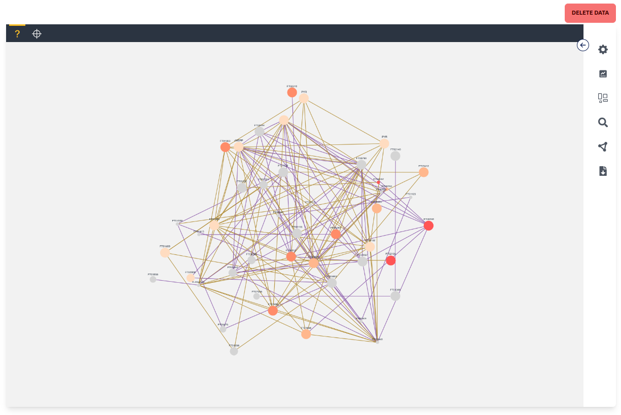
Unknown mode can potentially display every node available in the network graph based on the displayed nodes in a force-directed layout. Each node has a label, different size and color, as well as potentially multiple colored edges. Each label depends on the "name" given in the network graph, while the size and color depend on the chosen settings and are by default anova p-values between the different experiments where size maps to the quantity p-value and color to the labeling p-value. Each edge is at least one connection between two nodes in a single experiment where the color depends on the experiment. Nodes and edges can be clicked, which "selects" them and makes it possible to view Node Data and Edge Data respectively. Nodes can also be dragged around and the zoom can be changed with the mouse wheel.
Targeted mode can be used if MID data was mapped onto an optional pathway previously. The MID nodes that were linked to the pathway are now displayed on the pathway with the same visuals as in the Unknown Mode. Some settings are different for the Targeted and Unknown mode, which will be discussed in the specific sections.
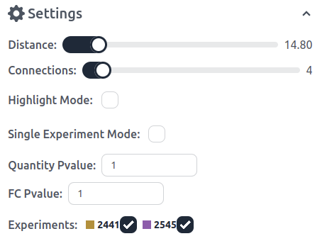
Distance: Each Edge has a minimum, maximum, mean, median, and scaled mean distance. The distance regulator filters edges based on their scaled mean distance (from 0 to 100).
Connections: Connections are grouped per experiment into a singular edge. This filters edges based on their total connections.
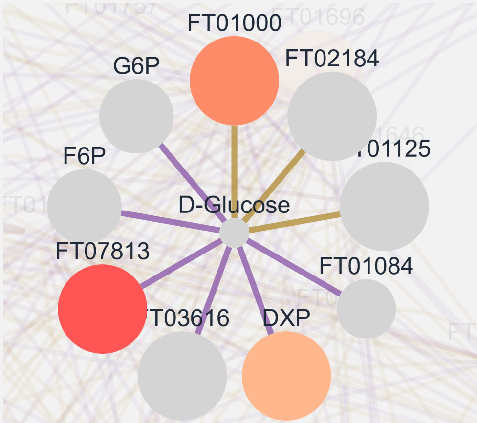
Highlight Mode: By default clicking on a node shows the node and all its connecting edges and nodes. Highlight mode in contrast "highlights" and brings all the nodes and edges into the foreground (see below). Clicking on a different connected node highlights said node and displays all its connected nodes. Targeted Mode: Targeted mode specifically only displays the pathway node. By using highlight in target mode all connected nodes are displayed even the ones not on the pathway map.
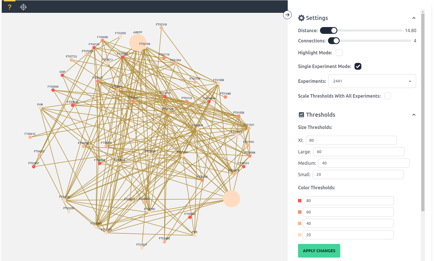
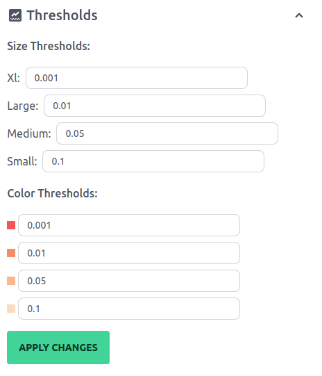
Single Experiment Mode: As the name suggests single experiment changes the display to a single experiment and also changes the color and size values displayed to a scaled fractional contribution and scaled quantity value respectively. The thresholds can be adjusted in the thresholds section. A new setting is also available Scale Thresholds With All Experiments, which if enabled scales the quantity and fractional contribution values together for all experiments.
Quantity and FC Pvalue: This options filters nodes below the given threshold. This option is disabled for Targeted Mode.
Experiments: Experiments filters edges based on their experiment. This option is not available in the Single Experiment Mode.
The thresholds tab makes it possible to change the thresholds of the different size and color classes. These values change from the anova p-value to the scaled quantity and fractional contribution in Single Experiment Mode.
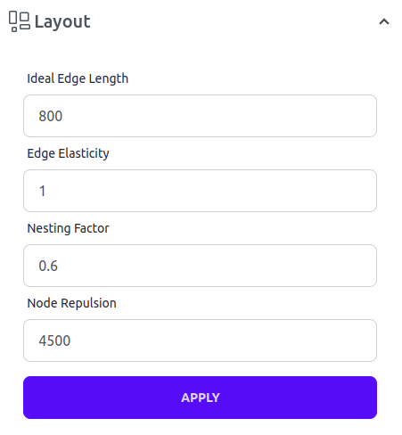
The layout tab is only available in unknown mode, which allows the user to change the parameters of the force-directed layout. The ideal parameters depend on the data that is used and should be played around with. For more details you can look at the documentation of the algorithm that was used, Cose-Bilkent.
The search tab allows users to search for the name of a node, if a node is clicked from the list it is selected for the purposes of the Metabolite Data tab and is clicked in the graph if present.
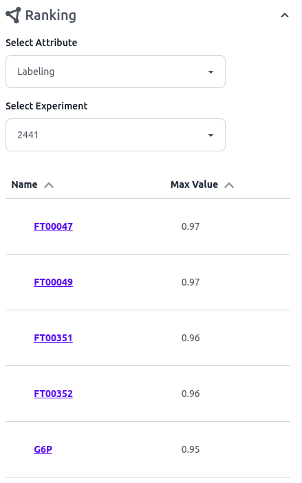
The ranking tab displays a list of all nodes included in the network graph, which can be sorted based on the maximum fractional contribution (Labeling) or the maximum pool size (Quantity) for each experiment. The name of each node can then be clicked to select it.
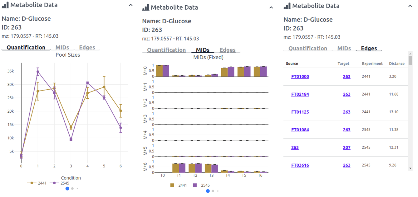
When/if a node is clicked on or selected the option Node Data appears. Node data displays the name, id, accurate mass and retention time of the given node. Below that are three tabs for additional info/figures. The first tab Quantification displays 3 quantification plots which can be clicked through with the blue balls below the figure. The first figure displays the pool sizes, the second figure the fractional contribution, and the third figure the pool size multiplied by the fractional contribution. The second tab MIDs also includes three figure which can be clicked through. The first a bar plot with a fixed axis, the second a bar plot zoomed based on the mass isotopomer, and the third a stacked bar plot for each experiment. The third tab Edges is a list of all edges belonging to that node, with the nodes source and target ids, the experiment and the scaled mean distance.
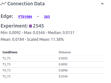
When/if an edge is clicked on or selected the option Edge Data appears. Edge data shows the nodes which belong to the edge, the experiment, and all the distance parameters. Below all the edge properties a list of all calculated connections is listed with all the conditions that were compared in the format condition 1_condition 2 and the distance.
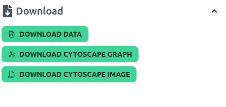
The full calculated dataset can be downloaded with the "Download Data" button. The current visible graph can be downloaded as a cytoscape graph in JSON format or as an image in PNG format with the respective buttons.
Every major IMPACT tool redirects to a "Job Page" during calculation of the diverse algorithms. Here you can see the progress of the server in handling your request with timestamped updates. You can close this page and come back to it any time you want. Just save the URL with the "Copy URL" button. After successfully running the calculation new buttons will appear below the update box where you can download the results or redirect to the next tool for further analysis.